Risa/Asir 2000
Risa/Asir can plot the planar algebraic curves with self intersections.
This feature is very usefull and powerfull comparing to the other CAS
( such as Mathematica and Maple ). Risa/Asir are included in
OpenXM and uses
OpenXM protocol to plot graphs etc .
Risa/Asir has a C-like language. But it doesn't have a notebook style
frontend. You can use "fep" to realize the emacs/vi-like command line
interface. "fep" is included in OpenXM. fep's options are "-emacs" or
"-vi". If you want use asir in emacs key binding,
startup asir with fep as the following:
fep -emacs asir
Ploting algebraic curves
Risa/Asir plots the graphs with the following steps:
- A client sends the message to the server.
- The server calculates.
- The client sends to server the message to pass the results.
- The server passes the results to the client.
To execute the distribute computing via OpenXM, you must launch
a server and establish the connection to it.
At first, you should execute ox_launch or ox_launch_nox command.
ox_launch is for the X11 environment, ox_launch_nox is
for the non-X11 environment. These command need the host id,
the directory and the command as arguments. The host id is 0
if the same computer that asir works on, and the directory is
where the command to execute is placed on. If the command is
on the ASIR's directory path, then you may omit it. For example,
you would plot the graph with ifplot on the X11-environment,
you should only input ox_launch(0,"ox_plot");.
If your environment is a unix, xterm comes up.
This xterm is for showing the logs. If you can't use the X11 system,
you can use ox_launch_nox whose arguments are the same of ox_launch.
If your X11 system is XFree86 4.3.0, then xterm may fail to launch.
This dues to the imcompleteness of the internationalization of X11.
You should set the locale to C or edit .Xdefaults and add the line
"XTerm*locale: false". The following example is the log of xterm,
when xterm comes up.
Asir-Contrib xm version 20010310. Copyright 2000-2001, OpenX
M Committers.
help("keyword"); ox_help(0); ox_help("keyword"); ox_grep("ke
yword");
     for help messages.
I'm an ox_plot, Version 20020301.
#0 Got OX_COMMAND SM_mathcap

#1 Got OX_COMMAND SM_popCMO
pop at 0

#2 Got OX_DATA -> data pushed
#3 Got OX_COMMAND SM_setMathcap
pop at 0
After the initialization with ox_launch, you can plot planar
algebraic curves with ifplot etc.
You can also use gnuplot via OpenXM. In this case,
you should load the packages to use gnuplot. To do this,
you can only execute gnuplot_start(). Later I would show the example.
Examples for ifplot,conplot,plot and plotover
I will show some examples of asir's plotting commands.
These commands are ifplot, conplot, plot and plotover.
These plots a 2D-graph of a given (two variables) polynomial.
ifplot
ifplot( f(x,y) (,[w1,w2],[x,x0,x1],[y,y0,y1],id,"TITLE") );
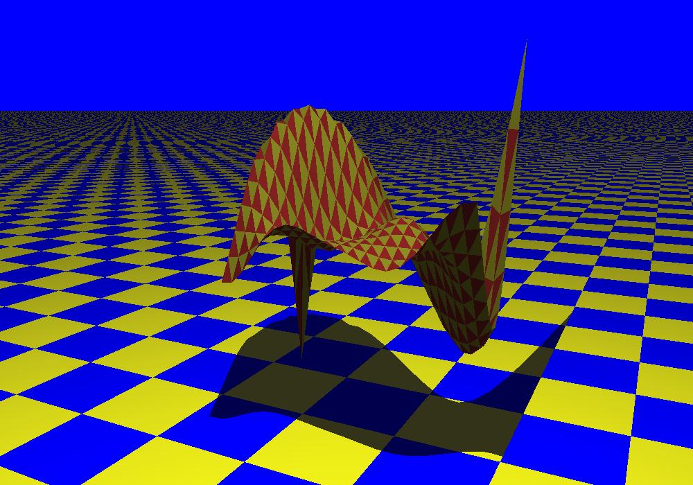
ifplot plots the zero set of 2 variable polynomial.
There are options in "()". The first [w1,w2] is the window's
size. If you don't use this option, it's efault window size
( 300x300 ) is used. [x, x0, x1] and [y, y0, y1] set
the ranges of the variables x and y. id is the number
which is set with ox_launch. if you would plot the graph
on the localhost, then this might be 0. The last "TITLE"
is the tiltle of the window.
|
An Example
[349] ifplot(x^3+x^2-y^2);
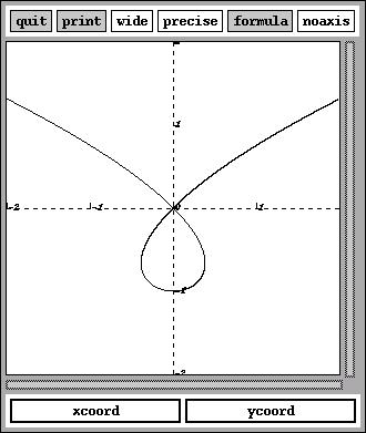
[350] ifplot(x^5-x*y^2+y^5,[x,-1,1],[y,-1,1],0,"Neko");
conplot
conplot(f(x,y) (,[w1,w2],[x,x0,x1],[y,y0,y1],[level,l0,l1],id,"TITLE"));
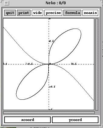
conplot generates the contour image of a given 2-variables
polynomial, i.e., for the given f(x,y), contplot plots
the ifplot images of f(x,y)+level ( where level is
a number of -2<=level <2, it's increment is 0.25 ).
This level can be set as an option.
|
Example
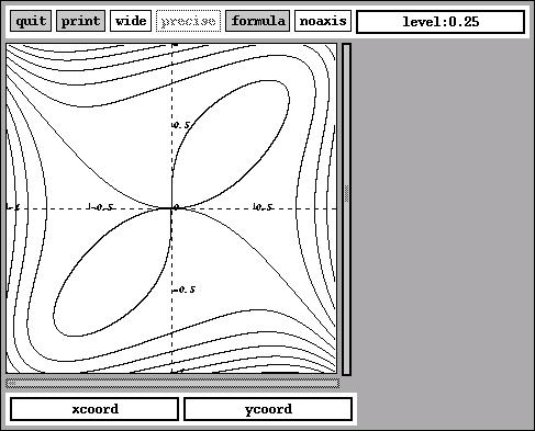
[350] conplot(x^3+x^2-y^2);
[351] conplot(x^5-x*y^2+y^5,[x,-1,1],[y,-1,1],0,"Neko");
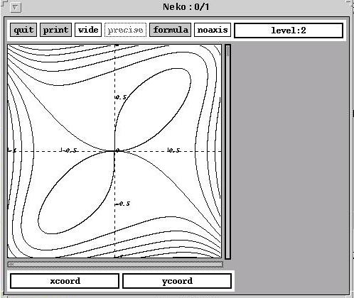
If you would operate the right-side scroll bar or push the bar,
the curve which is the specified level would be high-lighted and
it's level would be shown in the upper right level.
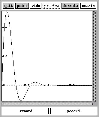
plot
plot(f(x) (,[w1.w2],[x,x0,x1],id,"TITLE"));
plot can show the graph of one-variable polynomial.
[w1,w2] sets the window size, [x,x0,x1] sets it's range,
id is the id of the server and "title" is the title of
the window.
|
Example
[355] plot(sin(2*x)*exp(-x),[x,0,10]);
plotover
plotover(function,id,"TITLE");
plotover add the new graph to the graph that is
plotted with plot, ifplot, conplot etc.
But the function should be the same type, one-variable
or two variables. For example, if you used plotover,
then the additional function must be one-variable and
if you used ifplot or conplot, then the polynomial must
be two variables.
|
Example
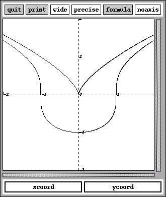
[360] ifplot(x^3-y^2+1);
0
[361] plotover(x^3-y^2,0,0);
0
[362]
Example
A very simple example. I show the cut-locus of the zero point set of
x^2*y^2+y^2*z^2+z^2*y^2-x*y*z with the plane x+y+z-k=0, where k is
a real number. The set is the following surface ( Steiner-Roman surface).

Steiner-Roman Surface ( generated by surf )
I plots the graphs which is the cut-locuses with the plane
x+y+z=K ( the normal vector is [1,1,1], [0,0,k] is included ).
So substitute z=k-x-y to the polynomial.
Definition of the function
def f(K) {
Z=K-x-y;
P=x^2*y^2+y^2*Z^2+Z^2*x^2-x*y*Z;
return P;
}
|
In the above programe, x and y are the indefinit variables and
Z and P is program variables. In Risa/Asir, the program variable
starts with the capital letter.
Example
[368] for (I=-5;I<=10;I++)
ifplot(f(0.1*I),[x,-0.6,0.6],[y,-0.6,0.6]);
[369]
|
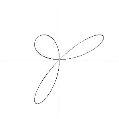
Execute the above, 15 windows come up. In each window, there is
an ifplot image. You can save these graphs as EPS files and convert
these files to a mpeg animation with convert included in ImageMagic
package. But the curves in these files are black only. It is not
so beautiful to see an animation. So you can modify these files
that the color of curve is red. The following is the part of
the file genereted with Risa/Asir.
Generated PostScript file ( part )
%%BoundingBox: 100 100 400 400
%%Creator: This is generated by ifplot
%%Title: ifplot
%%EndComments:
0.1 setlinewidth
2 setlinecap
2 setlinejoin
/ifplot_putpixel {
    /yyy 2 1 roll def /xxx 2 1 roll def
    gsave newpath xxx yyy .5 0 360 arc
    fill grestore
} def
 137 198  ifplot_putpixel
 137 199  ifplot_putpixel
(---Omitted---)
 323 344  ifplot_putpixel
 gsave [3] 0 setdash newpath
 249 100 moveto 249 400 lineto stroke
 stroke grestore
 gsave [3] 0 setdash newpath
 100 249 moveto 400 249 lineto stroke
 stroke grestore
showpage
|
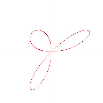
You can specify the color of curve with setrgbcolor. For example,
"l 0 0 setrgbcolor" sets the curves to be red.
I would set the curve to be red, axis to be black. To do so, I use
the following AWK script.
Script
#! /bin/sh
cat $1| awk '{print $0}
             /} def/{print "1 0 0 setrgbcolor";}
             /gsave \[3\]/{print "0 0 0 setrgbcolor";}'>tmp;
mv tmp $1;
|
This is an awk script. /pattern/{command1;command2;...}.
If there is "} def" in the stream, then adds "1 0 0 setrgbcolor"
in the line, if "gsave [3]" in the stream, then adds "0 0 0 setrgbcolor".
You can get that axes are black and curve is red.
The following is an example which translates EPS files to a mpeg file.
Example
Before
The after
Example
ponpoko@X20:~/asir > ls * | awk '/eps/{print "sh mkmk",$1}' >aa
ponpoko@X20:~/asir > sh aa; convert -density 100x100 *.eps asir.mpg
|
|
The mpeg file��asir.mpg
|
Surf - Examples from SuSE Linux Manuals.�˼�����MPEG�ե�����

The cut-locuses generated with Surf
The following script is for the above image.
If you are interested in it, please see
Surf - Examples from SuSE Linux Manuals.
Script for the above image
rot_x=-0.2;
rot_y=0.6;
rot_z=0.6;
origin_z=0;
scale_x=0.06;
scale_y=0.06;
scale_z=0.06;
illumination=ambient_light+
diffuse_light+reflected_light
+transmitted_light;
transparence=50;
clear_screen;
surface=x^2*y^2+x^2*z^2+y^2*z^2-x*y*z;
draw_surface;
plane=x+y+z-1;
curve_red=255;
curve_green=0;
curve_blue=0;
cut_with_plane;
plane=x+y+z-0.3;
curve_red=200;
curve_green=100;
curve_blue=0;
cut_with_plane;
plane=x+y+z;
curve_red=100;
curve_green=200;
curve_blue=100;
cut_with_plane;
plane=x+y+z+0.2;
curve_red=0;
curve_green=100;
curve_blue=255;
cut_with_plane;
plane=x+y+z+0.5;
curve_red=0;
curve_green=255;
curve_blue=0;
cut_with_plane;
|
To use GNUPLOT
RISA/ASIR can use GNUPlot via OpenXM. To use GNUPlot, execute
load("xm") and gnuplot_start(), you can use gnuplot with ordinal
gnuplot commands. The followings are an example.
Example
ponpoko@X24:~> asir
This is Risa/Asir, Version 20020301 (Kobe Distribution).
Copyright (C) 1994-2000, all rights reserved, FUJITSU LABORATORIES LIMITED.
Copyright 2000,2001, Risa/Asir committers, http://www.openxm.org/.
GC 5.3, copyright 1999, H-J. Boehm, A. J. Demers, Xerox, SGI, HP.
PARI 2.2.1(alpha), copyright (C) 2000,
C. Batut, K. Belabas, D. Bernardi, H. Cohen and M. Olivier.
Asir-Contrib xm version 20010310. Copyright 2000-2001, OpenXM Committers.
help("keyword"); ox_help(0); ox_help("keyword"); ox_grep("keyword");
for help messages.
[716] load("xm");
1
Asir-Contrib xm version 20010310. Copyright 2000-2001, OpenXM Committers.
help("keyword"); ox_help(0); ox_help("keyword"); ox_grep("keyword");
for help messages.
[900] gnuplot_start();
0
[901] gnuplot("plot sin(x**2);");
0
[902] gnuplot("splot (x**2+y**2)*sin(x**2+y**2)");
0
[903] gnuplot("set isosamples 50");
0
[904] gnuplot("splot (x**2+y**2)*sin(x**2+y**2)");
0
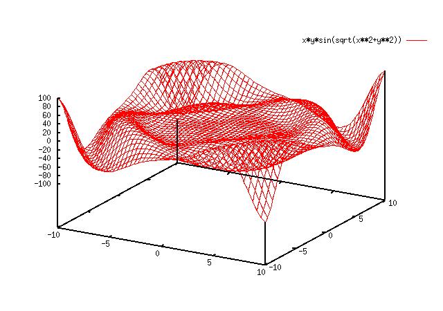
[905] gnuplot("splot x*y*sin(sqrt(x**2+y**2))");
0
|
In the above, gnuplot commands (plot, splot, set ...) were executed
with gnuplot command. For example, "plot" draws a curve and
"splot" draws a surface. The next image is generated by
"gnuplot("splot sqrt(x**2+y**2))".
For more infomation, please see OpenXM/lib/asir-contrib/gnulot.
To use povray
GNUPlot is very usefull, but gnuplot can't generate (rendered)
images like SURF which is for algebraic curves and surfaces
with singularities. For Risa/Asir, there are a package
that can generate a beautiful image using POVRAY.
But this is in the beta stage. This package is povray.rr
which can generate the image of surfaces of z=f(x,y).
You can load this with load("povray.rr").
At first, I show the example in povray.rr,
    povray_prolog("t.pov",0,0);
    povray_spheres(0,[ [0,3,0,3],[1,1,0,2] ]);
    povray_epilog(0);
|
I set the data file name (t.pov ) with povray_prolog,
then Asir opens the file. Next, povray_spheres generates
the sphere datas specified as lists, and povray_epilog
close the data file. But you can't get the image directly.
You should execute povray ( in the above example, execute
povrat +It.pov, then you can get t.png. ).
The following image is the rendaring image of t.pov.

In the above example, you shoud execute povray to generate
the image, but you can execute povray in asir directly.
Please see the example( test_mesh2 ) in povray.rr.
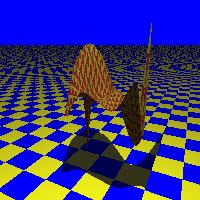
This test_mesh2 generates the rendering image:
povrat_plot3d_mesh is useful. This command generate the fixed name
file( t.pov) and ranges are fixed to [-5,5]x[-5,5]. And this command
adds the XY-Plane ( through (0,0) ), and this plane hides the object
that is Z<=0. In the following example, I show it's inputs and
output file( this is too long to see, so I show it as a part).
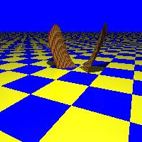
[744] povray_plot3d_mesh(x*y*sin((x^2+y^2)^(1/2))+25);
Z_bound=[13.6949,36.3051]
[[-5,-1],[5,5]]
 (t.pov) (w) file /asir_file_tmp set

(omitted)

@@@           @@@@@@@     ...........       ...@            @@@@@@@    @@@@@@
@@@@@@    @@@@@@@@@@@@        ....            ........    @@@@@@@@@@@@
@@@@@         @@@@             @@@@.....    .............         @@@@
@              @@@@@@@       @@@@@@@@@@@@.       .......              @@@@@@@
           @@@@@@@@@@@@@MM   MMMMMMMMMMM               @@@            @@@@@@@

Done Tracing
t.pov Statistics, Resolution 200 x 200
----------------------------------------------------------------------------
Pixels:           40000   Samples:           40000   Smpls/Pxl: 1.00
Rays:             67223   Saved:                 0   Max Level: 2/5
----------------------------------------------------------------------------
Ray->Shape Intersection          Tests       Succeeded  Percentage
----------------------------------------------------------------------------
Mesh                             97595            7394      7.58
Plane                            97595           31000     31.76
Sphere                           97595               0      0.00
Bounding Box                    571740          143115     25.03
----------------------------------------------------------------------------
Calls to Noise:                  0   Calls to DNoise:             10
----------------------------------------------------------------------------
Shadow Ray Tests:            91116   Succeeded:                 3569
Reflected Rays:              27223
----------------------------------------------------------------------------
Smallest Alloc:                 12 bytes   Largest:            26632
Peak memory used:           124484 bytes
----------------------------------------------------------------------------
Time For Trace:    0 hours  0 minutes   5.0 seconds (5 seconds)
    Total Time:    0 hours  0 minutes   5.0 seconds (5 seconds)

;
0
[746]
|
t.png
The default image size is 200x200. But you can generate the image
in the any size you want from it's data. To do this, you should specify
the size to povray. For example, if you want 1000x700 sized image,
then you should execute povray +It.png +W1000 +H700 ( t.png is
the datafile name).
povray_render only call povray with shell command. The following is
the definition of povray_render.
def povray_render(F)  {
   /* If FreeBSD, */
   shell("   povray +i"+F+" +L/usr/local/lib/povray3/include +D0 +P +H200 +W200&")$
}
|
povray_render generate 200x200 sized image. This settings are
"+H200 +W200". If you want 1700x1000 sized image,
you can redefine povray_render with replaced options "+H1700 +W1000".
It is interesting to create your own programs.
index
Ponpoko
Last modified: Wed Aug 20 09:18:42 JST 2003